Build1 publisher3 min readPublished
Deleting two terms from the tied-SAE gradient leaves the Oja update
A LessWrong post shows the Oja rule falling out of tied sparse-autoencoder descent once two terms are dropped, then reports a language-model test where an initialization change moved the backprop baseline more than the Hebbian gap it was meant to explain.
The Engineer · Build desk
What happened
- A LessWrong post argues that modern competitive Hebbian learning rules already train sparse autoencoders implicitly, and that the approximations they make are what leaves them worse at it.
- The test ran a SoftHebb-based encoder on 64-dimensional residual-stream activations from TinyStories-1M with 3,200 ReLU latents, five epochs per setup under five seeds.
- Standard backpropagation reached 0.929 explained variance, a Hebbian encoder with a trained decoder reached 0.615, and tied Hebbian decoding reached -0.520, below the mean-activation baseline under the reported metric.
- Tied-weight backpropagation scored 0.391 under the original initialization and exceeded 0.90 after that initialization changed, and the same change produced NaNs in the Hebbian setups.
Compiled by The EngineerSomething wrong?How this is made
Why it matters
- constraint Because the Hebbian setups produced NaNs under the initialization that works for tied backprop, there are no scores for both families at a shared starting point, and the reconstruction gap cannot be charged to any particular missing term.
- decision A team already running SAEs can now name what a Hebbian encoder leaves out of the gradient, so the question about adopting one becomes what dropping the encoder contribution and the cross-latent interactions buys them.
- exposure Anyone treating dictionary coverage or dead-feature fraction as an SAE health check would have ranked the worst reconstructor in this run first.
- precedent If the tied-weight identity holds up, storage-capacity results from the associative memory literature become arguable claims about SAE dictionaries, which is the reason the post gives for interpretability researchers to care.
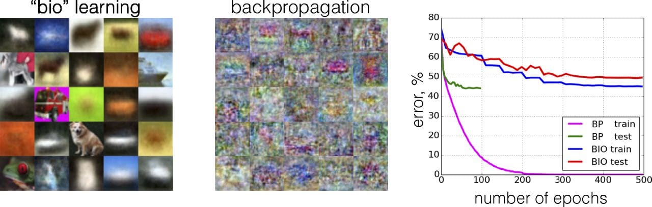
The conjecture starts with a 2019 paper, Unsupervised learning by competing hidden units, in which a linear layer trained on CIFAR-10 with a biologically inspired rule ended up with weights that resemble the input images or image prototypes; the post's authors took that neuronal selectivity to be analogous to the feature selectivity SAEs give language-model interpretability work [20].
Tying the weights is what lets the two objects be compared at all. One shared matrix means updating it updates the whole autoencoder, there is no second decoder matrix to train, and both uses of the matrix still contribute to its derivative [4]. The exact reconstruction anti-gradient has two terms, the first being the decoder contribution [5]. Drop the second, discard the off-diagonal entries, and each feature is left with the familiar Oja update [5]. Independent Oja updates therefore omit the encoder contribution and the cross-latent reconstruction interactions [6]. The post says of this step: "This is algebra, not an analogy." [7]
The sparsity side is looser. For a unit-norm weight vector and a positive activation, projected descent on an activation penalty and squared descent move along different directions, and the second is negative Oja [8]. In the narrow case of a tied ReLU SAE with one active latent, zero bias and unit-norm weights, the projected update is exact, with reconstruction attracting and the penalty repelling [9]. SoftHebb, from the ICLR 2023 paper, adds softmax coefficients and winner/loser signs that differ from ordinary SAE gradients, and the post states that these connections do not make its full update exact SAE descent [10]. The full derivations, the assumptions and corrections to the underlying paper, first published at the NFAM 2025 workshop, are in the appendix [19][22].
Initialization alone moved the tied backprop setup by at least 0.509 explained variance [1]. That is larger than the 0.314 separating standard backprop from the Hebbian encoder with a trained decoder [2], which is the gap the approximations are supposed to explain. The post is direct about the limit: "The experiment does not isolate which departure caused poor reconstruction." [17]
The dictionary statistics point the other way from the reconstruction column. On a 3,200-entry dictionary, 59 percent usage against 19 percent is about 1,890 entries against 610 [6], and roughly 22 active latents per input is about 0.7 percent of the dictionary [4]. Broad coverage reads as a healthy dictionary right up to the point where you check the reconstruction score. The post makes the same point in one line: "Broader dictionary usage does not itself establish better features." [16]
For that ranking to say anything about a production SAE, the ordering would have to survive residual streams much wider than 64 dimensions and an initialization tuned for both families. The dictionary here is 50 times the input width [3], the source model is TinyStories-1M [11], and the selected activation patterns were inspected on NeelNanda/pile-10k [21]. The post's own summary is that the results fit a hypothesis worth testing: the rules do something related to SAE optimization while departing from its exact updates [18].
What to watch
- A Hebbian run that survives the better initialization without NaNs would give the first same-init comparison against tied backprop's 0.90-plus score.
- An ablation restoring the encoder contribution and the cross-latent terms one at a time would say which deletion costs the reconstruction.
- The revised paper's appendix, which the post says holds the derivations, assumptions and corrections to the NFAM workshop version.